|
|
Please login with your username and your password. Select the module ‘Compression spring’ through the tree structure of the project manager by double-clicking on the module or clicking on the button ‘New calculation’.
Spring is a mechanical device designed to store elastic energy when deflected and to return the energy when relaxed. The compression spring offers resistance to a compressive force applied axially.
The calculation of the compression spring is based on DIN EN-13906-1. Forces and deflection or a combination of both parameters can be defined for the calculation. Other parameters for the spring geometry (e.g., length, diameter, coils) can be entered manually or can be selected from the geometry database according to DIN 2098. If you manually enter the parameters, you can define an individual compression spring. The depending values will be automatically calculated.
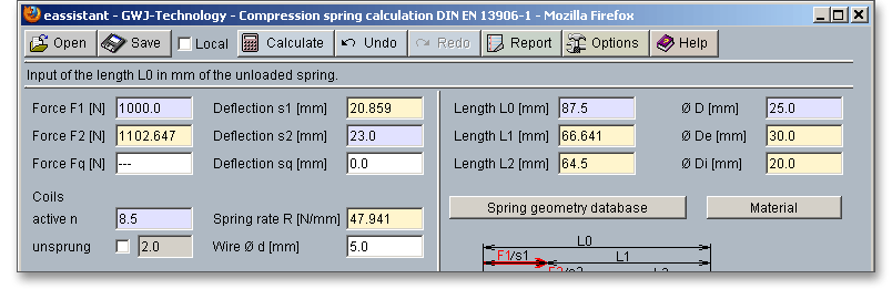
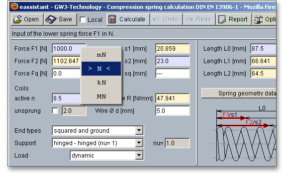
For the entry of forces and deflections there are the following possibilities:
|
|
||
|
|
||
|
|
||
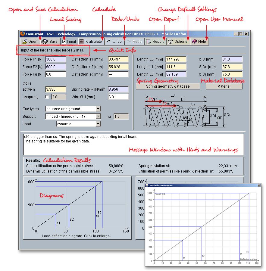
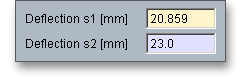
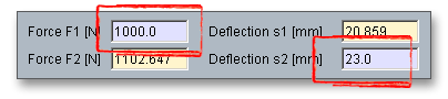
The input fields that are dependent upon one another are color-coded to simplify the connection of force,
deflection and length. Click the input field and the corresponding input field will turn yellow. It makes it easier for
you to see how these values relate to each other and how they change.
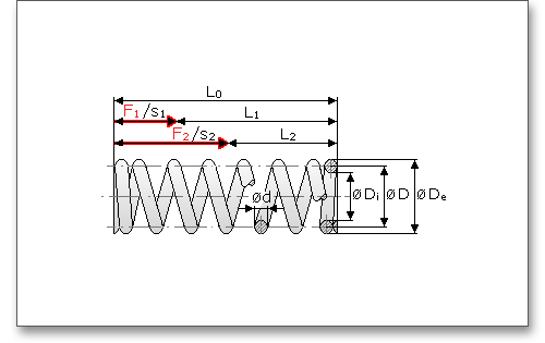
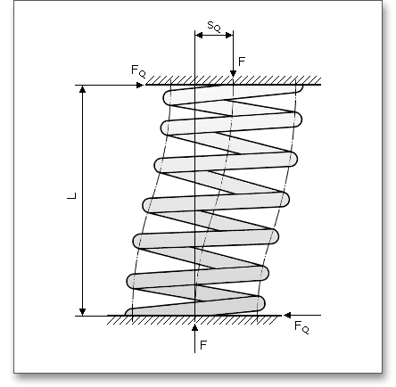
If an axially loaded spring with parallel guided ends is additionally perpendicular to its axis, transverse deflection with localised increase in torsional stress will occur (DIN EN 13906-1: July 2002, p. 10).
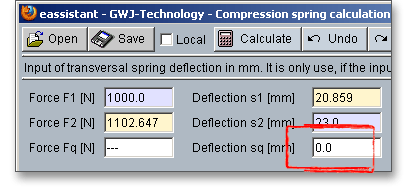
Enter either force or deflection in order to consider transverse loading.
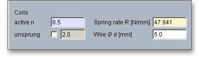
Enter the number of active coils  . The manual entry allows the dimensioning of individual compression
springs. Activate the option ‘unsprung’ and enter a value for the number of unsprung coils.
. The manual entry allows the dimensioning of individual compression
springs. Activate the option ‘unsprung’ and enter a value for the number of unsprung coils.
Enter either a value for the coils  or the spring rate
  . The input fields are color-coded. If you enter a
number of active coils, the spring rate is automatically determined and input field turns yellow. In case you define
the spring rate, the input field for the coils turns yellow.
. The input fields are color-coded. If you enter a
number of active coils, the spring rate is automatically determined and input field turns yellow. In case you define
the spring rate, the input field for the coils turns yellow.
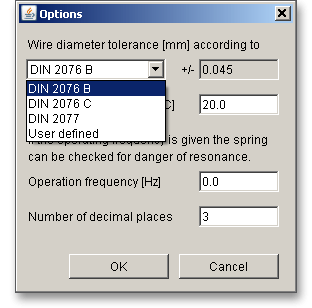
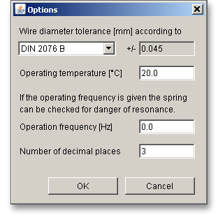
Please Note: Click the button ‘Options in order to consider the wire diameter tolerances. The listbox provides the tolerances according to DIN 2076 B/C and DIN 2077. Selecting the entry ‘User-defined’ allows you to define an individual wire diameter tolerance.
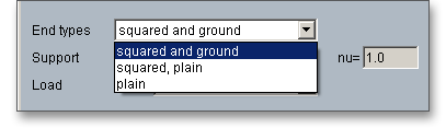
Select the following spring end types:
Some springs have the tendency to buckle. The critical spring length at whick buckling starts is known as the
buckling length  . The spring deflection up to the point of buckling is known as the buckling spring deflection
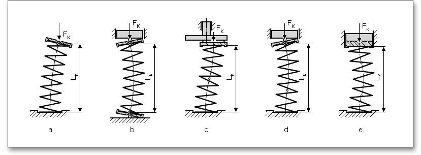
 . The influence of the seating of the spring ends is taken into account by means of the seating coefficient
 .
.
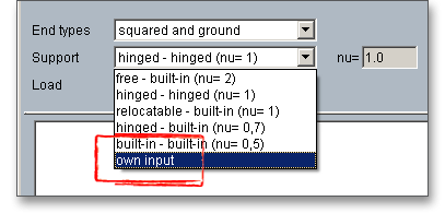
For the support of spring end types the following options are available:
 = 2)
= 2)
 = 1)
= 1)
 = 1)
= 1)
 = 0,7)
 = 0,5)
Please Note: Select the option ‘Own input’ and enter your own supporting coefficient  of the spring end
type.
of the spring end
type.
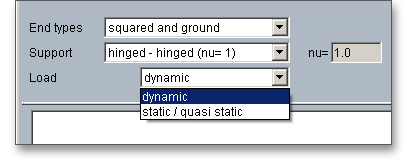
Before starting the calculation, it should be specified whether they will be subjected to static loading, quasi-static loading or dynamic loading. The calculation is possible for both dynamic and static/quasi-static loading. A static loading is:
Quasi-static loading is:
 fatigue strength)

In the case of compression spring dynamic loading is loading variable with time with a number of load cycles
over  and torsional stress range greater than 0,1
  fatigue strength at:
Depending on the required number of cycles  up to rupture it is necessary to differentiate between two
cases as follows:
up to rupture it is necessary to differentiate between two
cases as follows:
 for cold coiled springs
 for warm coiled springs
Torsional stress range is lower than the infinite life fatigue limit.
 for cold coiled springs
 for warm coiled springs
Torsional stress range is greater than the infinite life fatigue limit but smaller than the low cycle fatigue limit.
Enter the values for the length and diameter. The input fields that are dependent upon one another are color-coded. Click the input field and the corresponding input field will turn yellow. It makes it easier for you to see how these values relate to each other and how they change.
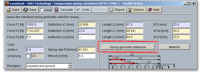
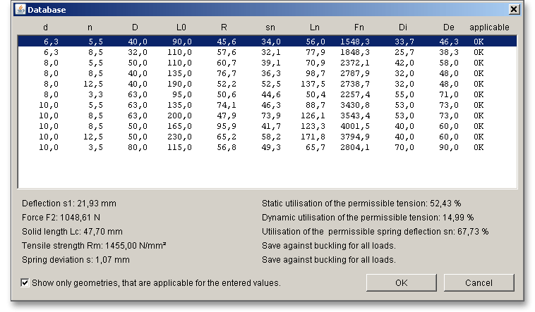
You can either enter the spring geometry with length, diameter and coils directly into the input fields or you can choose the geometry from the spring geometry database according to DIN 2098. The spring database makes it possible to quickly find the spring that will meet your requirements. Start with defining the loads and click the button ‘Spring geometry database’.
The database provides a list of all spring geometries that can be used for your application. Please choose a compression spring and click the ‘OK’ button.
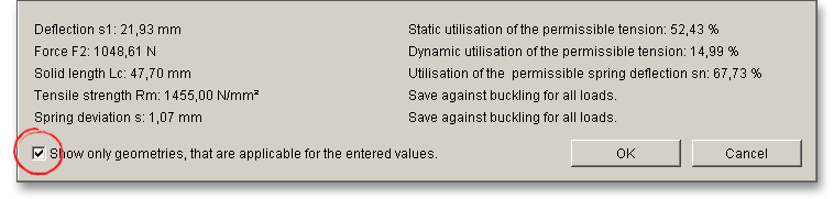
Please Note: The option ‘Show only geometries that are applicable for the entered values.’ is enabled by default. If you want to display all geometries, simply remove the checkmark from its box and select a spring geometry. Confirm with the ‘OK’ button.
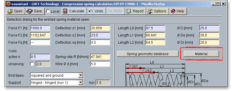
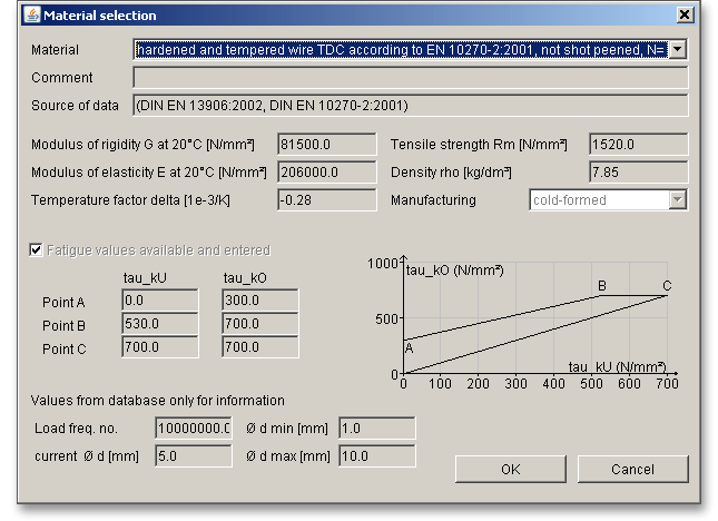
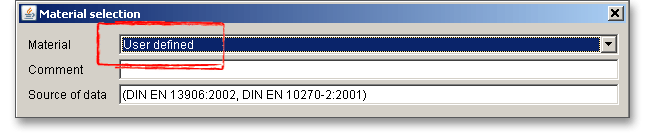
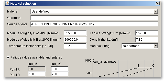
Clicking the button ‘Material’ opens the material database. In case there is no material that will fulfill the design requirements, then simply define your individual material.
Please select the material from the list. You will get detailed information on the material. The two cursor keys ‘Up’ and ‘Down’ of your keyboard allows you to navigate through the material database, so you can compare the different material properties with each other.
In case you cannot find the material you are looking for in our extensive database, simply define your individual material. You will find the entry ‘User-defined’ in the listbox. If you select this option, the input fields will be enabled, so that you can enter your own input values or add a comment. Depending on the manufacturing process (e.g., hot rolled or cold coiled springs), the calculation of the tolerances is determined according to DIN 2095 or DIN 2096. In addition, the eigenfrequency of the spring is calculated.
In order to confirm your inputs, click the button ‘OK’. Please be advised that changing the material will delete your defined inputs and you have to enter the inputs again.
Use this function if you want to change the unit of measurement quickly. Just a right-click on the input field where you want to change the unit. The context menu contains all available units. The two arrows mark the current setting. As soon as you select a unit, the current field value will be converted automatically into the chosen unit of measurement.
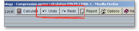
The button ‘Undo’ allows you to reset your input to an older state. The button ‘Redo’ reverses the undo.
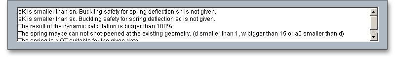
The calculation module provides a message window. This message window displays detailed information, helpful hints or warnings about problems. One of the main benefits of the program is that the software provides suggestions for correcting errors during the data input. If you check the message window carefully for any errors or warnings and follow the hints, you are able to find a solution to quickly resolve calculation problems.
The quick info feature gives you additional information about all input fields and buttons. Move the mouse pointer to an input field or a button, then you will get some additional information. This information will be displayed in the quick info line.
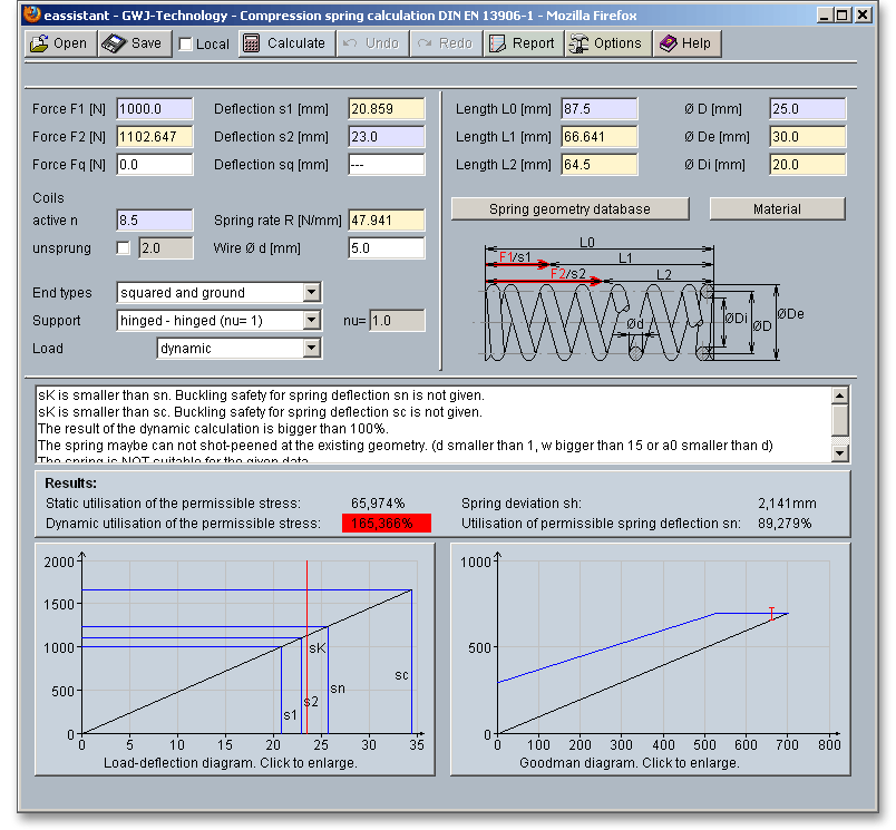
All important calculation results will be calculated during every input and will be displayed in the result panel. A recalculation occurs after every data input. Any changes that are made to the user interface take effect immediately. Press the Enter key or move to the next input field to complete the input. Alternatively, use the Tab key to jump from field to field or click the ‘Calculate’ button after every input. Your entries will be also confirmed and the calculation results will displayed automatically. If the result exceeds certain values, the result will be marked red.
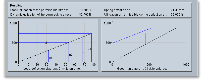
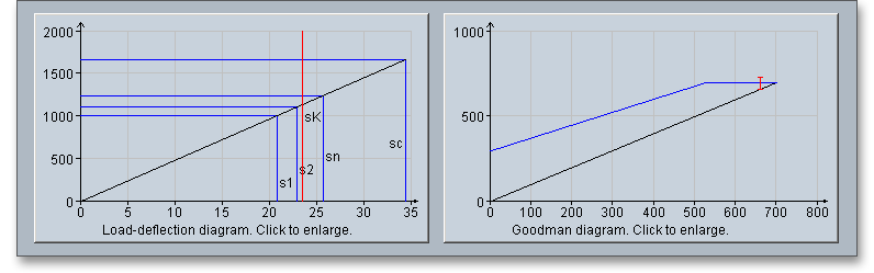
You get a graphical representation of the load-deflection and Goodman diagram. Click on the diagram to see the full image and details. The Goodman diagram is displayed only for the dynamic load.
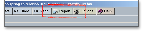
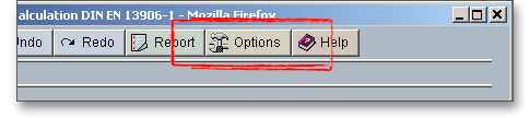
After the completion of your calculation you can create a calculation report. Click on the ‘Report’ button.
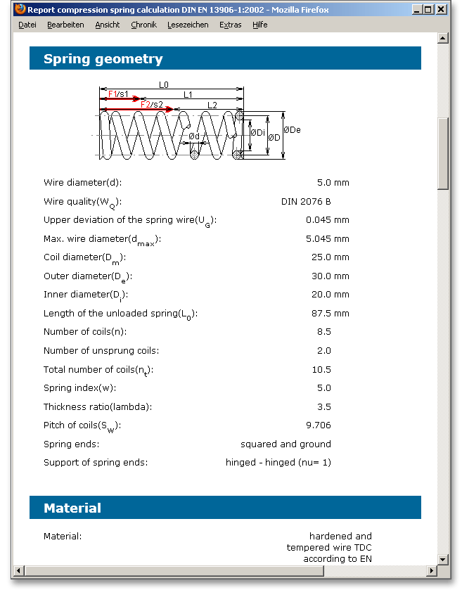
You can navigate through the report via the table of contents that provides links to the input values, results and figures. This calculation report contains all input data, the calculation method as well as all detailed results. The report is available in HTML and PDF format. The calculation report saved in HTML format, can be opened in a web browser or in Word for Windows.
You may also print or save the calculation report:
 ‘Save as’ from your browser menu
bar. Select the file type ‘Webpage complete’, then just click on the button ‘Save’.
‘Save as’ from your browser menu
bar. Select the file type ‘Webpage complete’, then just click on the button ‘Save’.
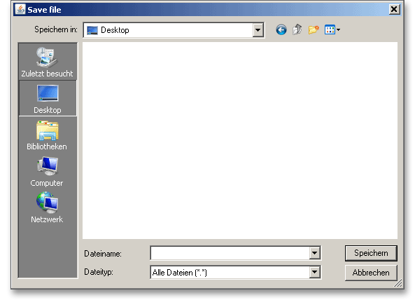
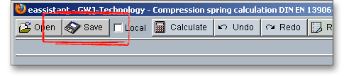
When the calculation is finished, you can save it to your computer or to the eAssistant server. Click on the button ‘Save’.
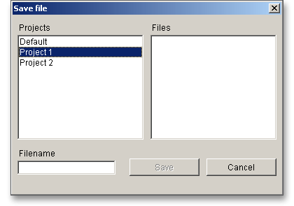
Before you can save the calculation to your computer, you need to activate the checkbox ‘Enable save data local’ in the project manager and the option ‘Local’ in the calculation module. A standard Windows dialog for saving files will appear. Now you will be able to save the calculation to your computer.
In case you do not activate the option in order to save your files locally, then a new window is opened and you can save the calculation to the eAssistant server. Please enter a name into the input field ‘Filename’ and click on the button ‘Save’. Then click on the button ‘Refresh’ in the project manager. Your saved calculation file is displayed in the window ‘Files’.
Click the button ‘Options’ in order to change the default settings.
Here are the default settings that you can modify:
Please login with your username and your password. Select the module ‘Compression spring’ through the tree structure of the project manager by double-clicking on the module or clicking on the button ‘New calculation’.
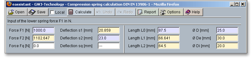
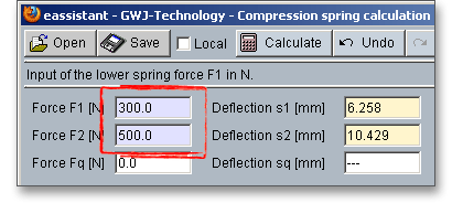
A cold coiled compression spring 4 x 32 x 120 is made of patented cold drawn spring steel wire
Wire diameter  | = 4 mm |
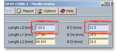
Diameter  | = 32 mm |
Coils  | = 8.5 |
Length of the unloaded spring  | = 120 mm |
| is alternately loaded with |
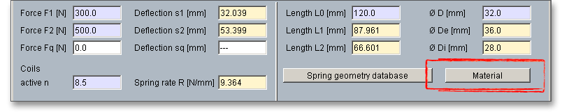
Spring force  | = 300 N |
Spring force  | = 500 N |
We are looking for the spring rate  , the corrected shear stress
  for the spring force
  = 500 N and
spring deviation
= 500 N and
spring deviation  .
.
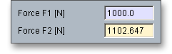
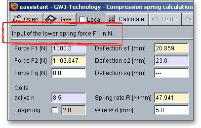
Please start to enter the spring forces  and
and  . During entering the spring forces, the corresponding
spring deflections are automatically determined and will be highlighted in a different color.
. During entering the spring forces, the corresponding
spring deflections are automatically determined and will be highlighted in a different color.
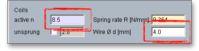
Enter the number of coils  as well as the wire diameter
  . The settings for the spring ends, the support of
spring as well the load will not be changed.
. The settings for the spring ends, the support of
spring as well the load will not be changed.
Enter the spring length  and the spring diameter
  .
.
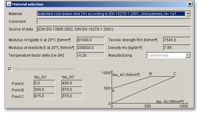
Click the button ‘Material’ to open the material database and to find the required material for the compression spring.
Select the following material from the listbox: patented cold drawn wire DH according to EN 10270-1: 2001, shot
peened,  .
.
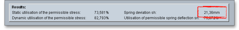
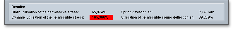
All important calculation results, such as the static and dynamic utilization of the permissable stress, the spring
deviation  and the utilization of the permissable spring deflection
  , will be calculated during every input
and will be displayed in the result panel. A recalculation occurs after every data input. Any changes that are
made to the user interface take effect immediately. Press the Enter key or move to the next input field to
complete the input. Alternatively, use the Tab key to jump from field to field or click the ‘Calculate’
button after every input. Your entries will be also confirmed and the calculation results will displayed
automatically.
, will be calculated during every input
and will be displayed in the result panel. A recalculation occurs after every data input. Any changes that are
made to the user interface take effect immediately. Press the Enter key or move to the next input field to
complete the input. Alternatively, use the Tab key to jump from field to field or click the ‘Calculate’
button after every input. Your entries will be also confirmed and the calculation results will displayed
automatically.
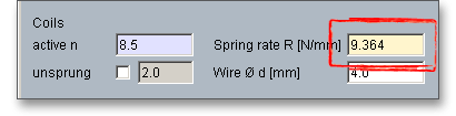
The spring rate  is = 9,364 N/mm and is displayed above the input field for the wire diameter.
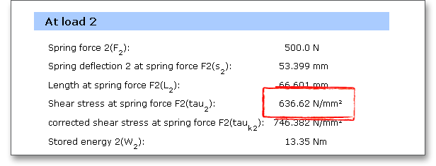
The calculation report provides the result for the shear stress. Click the button ‘Report’ to open the calculation
report. The shear stress  for the spring force
  is = 636,62 N/mm
 .
.
You will find the value for the spring deviation  in the result panel. The spring deviation
  is = 21,36
mm.
is = 21,36
mm.
The results are clearly displayed in the diagrams. Click on the diagram to see the full image and details.
After the completion of your calculation, you can create a calculation report. Click on the ‘Report’ button.
You can navigate through the report via the table of contents that provides links to the input values, results and figures. This calculation report contains all input data, the calculation method as well as all detailed results. The report is available in HTML and PDF format. The calculation report saved in HTML format, can be opened in a web browser or in Word for Windows. You may also print or save the calculation report:
 ‘Save as’ from your browser menu
bar. Select the file type ‘Webpage complete’, then just click on the button ‘Save’.
‘Save as’ from your browser menu
bar. Select the file type ‘Webpage complete’, then just click on the button ‘Save’.
When the calculation is finished, you can save it to your computer or to the eAssistant server. Click on the button ‘Save’.
Before you can save the calculation to your computer, you need to activate the checkbox ‘Enable save data local’ in the project manager and the option ‘Local’ in the calculation module. A standard Windows dialog for saving files will appear. Now you will be able to save the calculation to your computer.
In case you do not activate the option in order to save your files locally, then a new window is opened and you can save the calculation to the eAssistant server. Please enter a name into the input field ‘Filename’ and click on the button ‘Save’. Then click on the button ‘Refresh’ in the project manager. Your saved calculation file is displayed in the window ‘Files’.
Our manual is improved continually. Of course we are always interested in your opinion, so we would like to know what you think. We appreciate your feedback and we are looking for ideas, suggestions or criticism. If you have anything to say or if you have any questions, please let us know by phone +49 (0) 531 129 399-0 or email eAssistant@gwj.de.

 and wire diameter